Authored by: CA Punit Khandelwal
Assisted by: Sarthak Garg
“Valuation models are another area of finance that need to be tweaked in a negative rate environment. Nobel prizes have been awarded to economists that developed concepts such as the efficient frontier, the Capital Asset Pricing Model and the Black-Scholes option pricing model. But when a negative value is assumed for the risk-free rate in these types of models, fair value results shoot off toward infinity. With trillions of securities and derivatives dependent on these models, valuation is critical...”
- Jim Bianco, wrote this in the article, ‘Negative Interest Rates Threaten the Financial System’, dated 30 September 2019, https://www.bloombergquint.com/gadfly/negative-interest-rates-threaten-the-financial-system
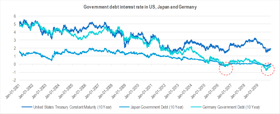
Large economies like Japan and Germany have been witnessing negative yields on government bonds since 2017. For example, 10-year zero-coupon sovereign bonds in Japan and Germany are trading at a yield of -0.14% and -0.46% respectively. The unorthodox monetary measures adopted by such economies which are aimed at deploying excessive reserves to spur growth has led various central banks to follow suit by aggressively reducing their interest rates. For example, the US is not too far with the Fed cutting the interest rates three times in 2019 to coax economic growth and balance its global trade wars. Such an economic environment where nominal interest falls below zero per cent raises an important question – how should the artificially suppressed extraneous short-term risk-free rate be factored in the computation of discount rates or the capitalisation rates?
Since negative interest rates essentially push the concept of a risk-free return to the extreme, it is critical to determine the return by benchmarking it to a normalised risk-free return of other economies which exhibit similar credit risk profile. The problem gets also accentuated due to low-level comfort of evaluators who tend to restrict themselves from using cash flow models in negative interest rate economies as it reduces discount rates considerably, consequently resulting in the model risking the possibility of not reflecting the fair value. This suggests that there might be a need to also evaluate other models for determining proxies of risk-free rate when the long term sovereign bonds are negative as shown in chart 1 below.

In the following paragraphs, we have discussed the various globally acceptable alternative economic models for determining proxies of the risk-free rate of negative interest rate economies.
Stress-testing the risk-free rate based on the Globally acceptable approaches
Evaluating alternative models for finding the best proxies to risk-free rate (in an adverse interest rate scenario) is essential because a lower risk-free rate (driven by market forces of high demand and quantitative easing policies of the central banks in these countries ) would result in a lower discount rate and consequently result in an artificially inflated asset valuation.
Alternative economic models that one may consider, among others, are –
- International Fisher Relation,
- Taylor’s rule,
- Others
- Long term borrowing rate of the largest firm adjusted for default risk and
- Normalised risk-free rates
International Fisher Relation
Under real interest rate parity, real interest rates are assumed to converge across different markets. Taking the Fisher relation and real interest rate parity together gives us the international Fisher effect:
Rnominal A – Rnominal B = E(inflationA) – E(inflationB)
The relation tells us that the difference between the two countries’ nominal interest rates should be equal to the difference between their expected inflation rates. The argument for the equality of real interest rates across countries is based on the idea that with free capital flows, funds will move to the country with a higher real rate until real rates are equalised.
Therefore, using the international Fisher effect, you can compute the nominal rate of return for Japan and Germany in comparison to the US using this formula:
Rnominal Japan = Rnominal US + {E(InflationJapan) – E(InflationUS)}
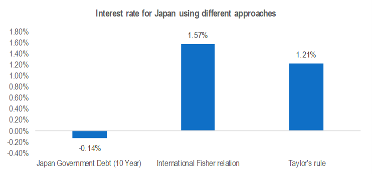
= 3% + {1.3%-2.73%} = 1.57%[1]
Rnominal Germany = Rnominal US + {E(InflationGermany) – E(InflationUS)}
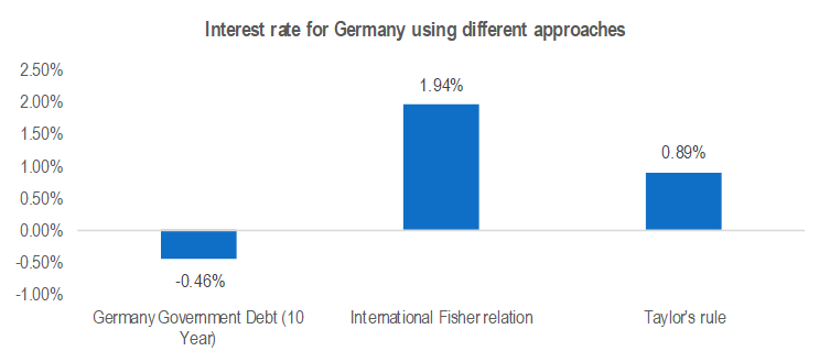
= 3% + {1.67%-2.73%} = 1.94%
Note: Inflation expectation for the year 2020 has been considered
Taylor’s rule
Taylor’s is used as a prescriptive tool (i.e., it states what the central bank should do). It also is reasonably accurate at predicting central bank action.
The Taylor rule determines the target interest rate using the neutral rate, expected GDP relative to its long-term trend, and expected inflation relative to its targeted amount. It can be formalised as follows:
ntarget = rneutral + itarget + [0.5(GDPexpected − GDPtrend) + 0.5(iexpected − itarget)]
where:
ntarget = target nominal short-term interest rate
rneutral = neutral real short-term interest rate
GDPexpected = expected GDP growth rate
GDPtrend = long-term trend in the GDP growth rate
iexpected = expected inflation rate
i target = target inflation rate
Applying Taylor’s rule – Japan
ntarget = rneutral + itarget + [0.5(GDPexpected − GDPtrend) + 0.5(iexpected − itarget)]
=-0.068% + 2.0% + [0.5(0.47% - 1.2%) + 0.5(1.3% - 2.0%)]
= 1.21%[2]
Applying Taylor’s rule – Germany
ntarget = rneutral + itarget + [0.5(GDPexpected − GDPtrend) + 0.5(iexpected − itarget)]
=-0.4562% + 2.0% + [0.5(1.25% - 2.2%) + 0.5(1.67% - 2.0%)]
= 0.89%[3]
[1] Source
Rnominal US: US Normalized risk-free rate from Duff & Phelps https://www.duffandphelps.com/insights/publications/valuation/us-normalized-risk-free-effective-september-30-2019
E(InflationJapan): Year 2020 estimate from Statista https://www.statista.com/statistics/270095/inflation-rate-in-japan/
E(InflationUS): Year 2020 estimate from Statista https://www.statista.com/statistics/244983/projected-inflation-rate-in-the-united-states/
E(InflationGermany): Year 2020 estimate from Statista https://www.statista.com/statistics/375207/inflation-rate-in-germany/
[2] Source
rneutral: Taken as Call Rate, Uncollateralized Overnight, Average (Daily) as on 31 December 2019 http://www.stat-search.boj.or.jp/ssi/mtshtml/fm01_d_1_en.html\
GDPexpected: Year 2020 estimate from Statista https://www.statista.com/statistics/263607/gross-domestic-product-gdp-growth-rate-in-japan/
GDPtrend: Taken as median of GDP growth rate from year 2006 to 2018 (World Bank national accounts data, and OECD National Accounts data files)
iexpected: Year 2020 estimate from Statista https://www.statista.com/statistics/270095/inflation-rate-in-japan/
[3] Source
rneutral: Taken as Call Money/Interbank Rate for Germany as on December 2019 (From OCED)
GDPexpected: Year 2020 estimate from Statista https://www.statista.com/statistics/375203/gross-domestic-product-gdp-growth-rate-in-germany/
GDPtrend: Taken as median of GDP growth rate from year 2006 to 2018 (World Bank national accounts data, and OECD National Accounts data files)
iexpected: Year 2020 estimate from Statista https://www.statista.com/statistics/375207/inflation-rate-in-germany/
i target: https://www.ecb.europa.eu/mopo/html/index.en.html


Other approaches
- Long term borrowing rate of the largest firm adjusted for default risk
Look for the largest and safest firms in the market and use the rate that they pay on their long-term borrowings in the local currency as a base. Given that these firms, despite their size and stability, still have default risk, consider a rate that is marginally lower than the corporate borrowing rate for determining the risk-free rate.[1]
- Normalised risk-free rates
Normalise risk-free rate by replacing the current (negative) interest rate with a reasonable risk-free rate, obtained from either history or fundamentals.[2]
Considering a 5-year average risk-free rate for the period 1 January 2015 to 31 December 2019, the risk-free rate based on this empirical data for Japan and Germany is 0.081% and 0.268% respectively.[3]
[1] Source Damodaran http://people.stern.nyu.edu/adamodar/pdfiles/blog/NegativeIntRates.pdf
[2] Source Damodaran http://people.stern.nyu.edu/adamodar/pdfiles/blog/NegativeIntRates.pdf
[3] Source Proprietary databases
Conclusion
Gazing at negative interest rates, we are of the view that valuation principles could be antagonised by temporal dimensions of interfered risk-free rates in growth-deflated big economies.
Based on the analysis of the alternative models which we have applied in two sample geographies, Japan and Germany, we note that an upward adjustment to the negative yields for 10-year zero-coupon sovereign bonds may be required for computing risk-free rate for the purpose of business valuations. Such adjusted risk-free rate would assist in ensuring that the asset prices are not artificially inflated and help in computing the fair value of such assets.

